
Bloom Filter - Part 2

Introduction
In this article, we will learn about the probabilistic nature of a Bloom filter and understand its speed and time complexity. I recommend reading the first article, Bloom Filter—Part 1, for an introduction to Bloom filters.
The probabilistic nature of the Bloom filter
The probabilistic nature of a bloom filter comes from the trade-off between space efficiency and accuracy. This space efficiency comes at the cost of allowing this data structure to return a “False-Positive” result. A “False-Positive” happens when a Bloom filter incorrectly tells that an element is available in the set.
Why does False-Positive happen?
When we map a data element to an index in a bit-array, the modulo operator restricts the index number generation from 0 to m — 1, where m is the size of the bit array. So, for an array of 20 bits, the indices range from 0 to 19.
Now, if I use one hash function to map 15 elements in a bit array of size 20, more than one element may map to the same index. When two elements map to the same index, it is called a collision or overlapping.
Because of this overlapping, when I search for a data element not added to the Bloom filter, it may map to an index with a value of 1.
(You can try this by modifying the variable bit_array_size to 10 or 15. Observe the collision when new elements are added. Refer — /For Articles/Bloom Filter — Part 1/simple_bloom_filter.py file. Available on GitHub as part of the first article.)
Managing bit-array size
One obvious way to minimize the collision is to increase the size of a bit array. But how much should I increase the size? This depends on…
a. How much data does this Bloom filter is expected to contain? Consider the data available for insertion and the rate of growth of this data in the near future. This is represented as n.
b. How many hash functions will I use to map a data element to different indices? Is there any recommendation on this number?
c. What is the probability of an error (“False-Positive”) that I am comfortable with? This is represented as P.
So, when I need a bloom filter, I’d think, “I need a bloom filter to manage 100K elements (n = 100K), and I am comfortable with an error rate of 1% (“False-Positive” of 1 out of 100 is manageable). (P = 1%)”
Formulas are available to calculate these values to ease our work. We should have a fair idea of the expected data (n) and the error rate (P) to calculate the size of a bit-array (m).
The formula is

m is the suggested size of bit-array.
n is the approximate number of inputs
P is the expected False positive rate
ln is called the natural logarithm. It refers to the log to base e.
When we know m (suggested size of bit array) and n (expected number of inputs), we can calculate k (expected number of hash functions) using the following formula.

So, for a bloom filter to manage 100K elements (n = 100K) with an error rate of 1% (“False-Positive” of 1 out of 100) (P = 1%)”, the expected size of bit-array is
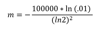
m = 958506. We need a bit-array of size 958506. This should easily accommodate 100,000 elements and have an expected error rate of 1%.
The expected error rate will increase if we add more data to this bit-array.
The recommended number of hash functions needed for this is
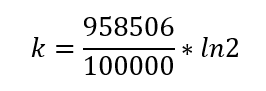
k = 7.
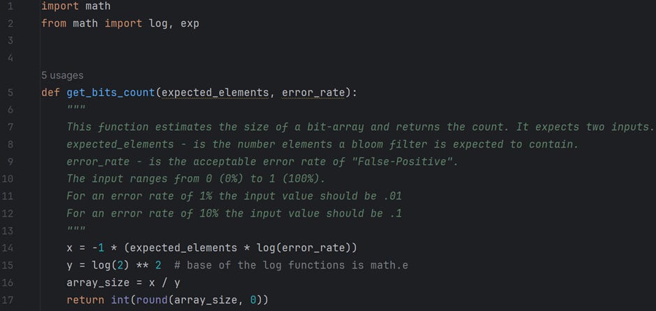
Code implementation
The above calculations are coded in Python and available in the file /For Article/Bloom filter — Part 2/measurements.py on GitHub. Please feel free to play around with the code. The following is a snapshot of the functions; the documentation explains their functionality quite well.

Revisiting False-Positive
Now, we know how to calculate the bit-array size based on the expected number of entries in a Bloom filter, the acceptable error rate, and the required number of hash functions.
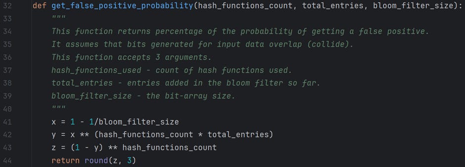
How do we know a Bloom filter’s false positive rate when adding entries? We have a formula for this, too.

m — is the number of elements in an array
n — is the number of values added to the array
k — is the number of hash functions used
The following table gives a fair idea of how a change in its attributes affects the “False-Positive” rate.

Following is the code snippet that implements the above formula.
Feel free to experiment with the code in the file /For Article/Bloom filter — Part 2/measurements.py on GitHub.
New Bloom filter class
With the above information, I will implement a new class for the Bloom filter. The constructor of this class expects two inputs: the expected entries of the Bloom filter and the acceptable error rate. Based on this, the class decides on the size of the bit array and the count of the hash function. This code is available in the folder /For Articles/Bloom Filter — Part 2/ on GitHub.
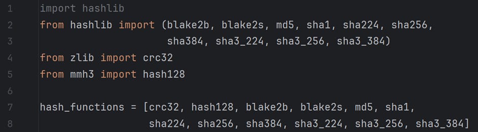
Since we will need many hash functions, I have enlisted various hash functions that the Python library hashlib provides. I have also used zlib for crc32 and mmh3 for the hash128 function. These are mentioned in the file /For Articles/Bloom Filter — Part 2/hashes.py on GitHub. Refer to the code snippet below.
Now, we will go through the implementation of the class BloomFilter in the file /For Articles/Bloom Filter — Part 2/bloom_filter.py on GitHub.
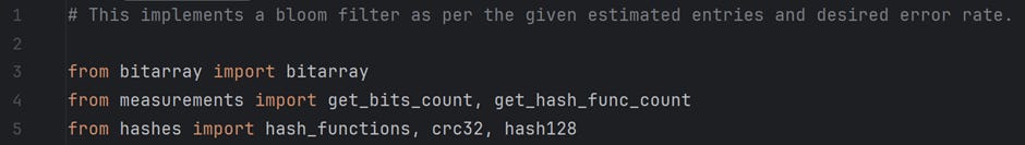
We start by importing bitarray module, which implements a bit-array. From the measurements module, we import two functions: get_bits_count and get_hash_func_count. The functionality of these two functions has already been explained above. Finally, from the hashes module, we import an array of hash_functions. This array has the names of all the hash functions available for use.
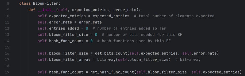
A user must pass two inputs while creating an object of the BloomFilter class. The expected number of entries to add to this bloom filter and the acceptable error rate of this data structure. Following is an explanation of each attribute defined in the class’s __init__().
expected_entries — stores the count of the total number of entries this data structure is expected to have. A user provides this input.
error_rate — is the acceptable error rate at which this data structure can operate. The value ranges from 0 (0%) to 1 (100%). A user provides this input.
entries_added — is the count of entries added in this data structure at a given time. This value increments as and when a new value is added.
bloom_filter_size — is a calculated field. It is the number of bits a bit-array should have to support the “expected_entries” at a given “error_rate.”
bloom_fliter_array — is the bit-array that contains all the data.
hash_func_count — is a calculated field. It is the count of hash functions this data structure must use to support the “expected_entries” at a given “error_rate.” Note that this program limits the number of hash functions available to 12.
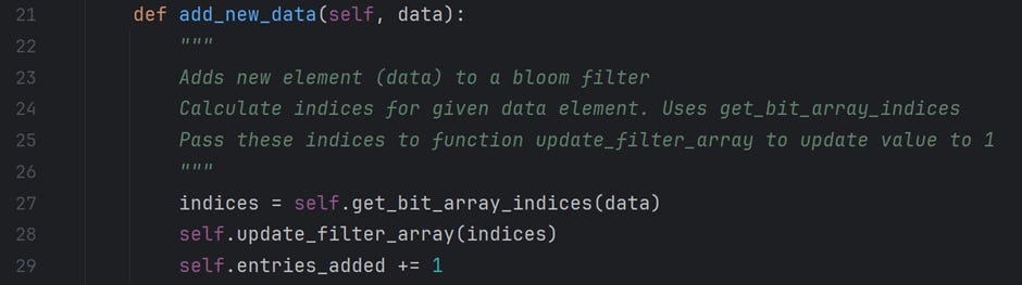
This method is responsible for adding new data elements to the bloom filter. To do this, it calls the function “get_bit_array_indices” to map the indices against the given data. Then, it updates the bloom filter array indices with the value 1 and increments the entries_added attribute. Now, we will get into the details of the function “get_bit_array_indices.”
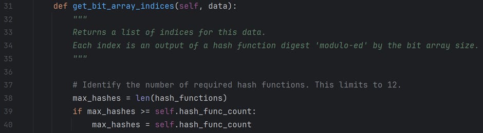
In the above section, we decide on the hash functions required for this data structure. There are a maximum of 12 available hash functions. If the hash_func_count is less than 12, we use the first hash_func_count function to calculate indices for a given data element.
For example, when we create a bloom filter with an expected_count of 100 and an acceptable error_rate of 1%, the program suggests a bit_array of size (m = 959) bits and hash_func_count of (k = 7). I will use this example in the upcoming sections to explain the code functionality.
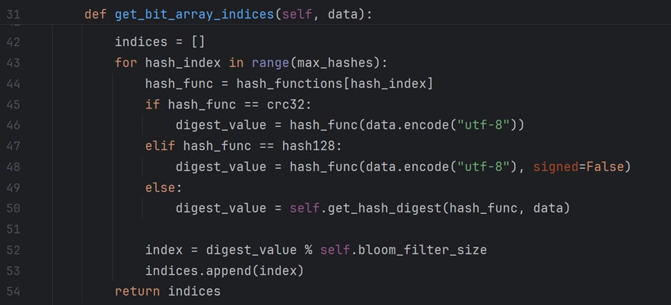
In this section of the code, I execute a for loop to execute the hash functions and calculate the index values for the data element. In this example, the max_hashes value is set to 7. So, the first 7 functions enlisted in the array “hash_functions” will be used to calculate indices.
Note: I have used crc32 and hash128 functions from different modules; hence, their execution style differs from the rest of the functions I have imported from the hashlib module. The function get_hash_digest executes the hash functions from the hashlib library.
All of these hash functions return an integer value, the hash_digest. The hash_digest is then “modulo-ed” by the bit-array size to calculate the index of an array. The indices are returned to the calling method “add_new_data.”
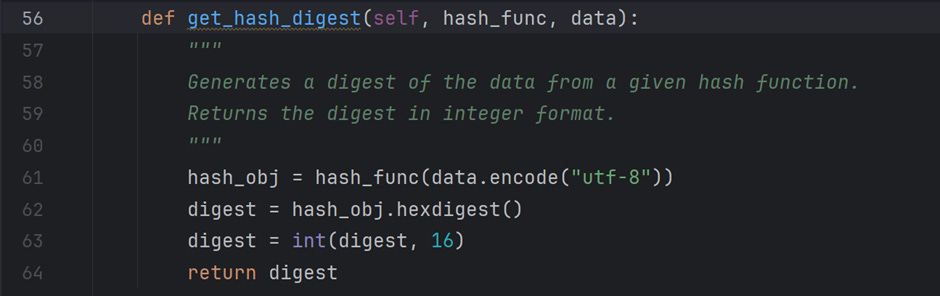
As mentioned, the function get_hash_digest executes the functions imported from the module hashlib. It starts by encoding the data value in “UTF-8” format and passing this string to a hash_func that returns a “hash” object. I gather the digest or hash value in hexadecimal format from this hash object and return it after converting it to an integer value.
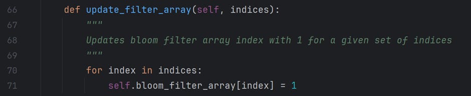
The method update_filter_array updates the index value of the bit-array to 1 for given indices.
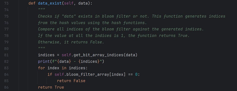
Once the data is inserted, I have written a method, “data_exist,” to search for a data element in an array.
I start by calculating the indices of the data value using the same set of hash functions used while inserting data into the data structure.
Every index is then checked in the bit array.
If any index value is 0, the function returns False, indicating that the data value does not exist.
Otherwise, the function returns True, indicating a data value in the data structure. Refer to the code below.
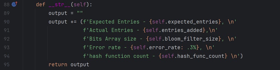
The last method is __str__(). This prints the details of a Bloom Filter object, which is useful while playing around with and debugging the code.
In addition, two more files are available in the source code.
The first is input_data.py, which contains the data this program inserts and searches for. It contains two lists: marvel_characters, which is inserted into the data structure, and DC_characters, which we search for in the data structure.
The second file is test_bloom_filter.py. It contains the code to test the functionality of the class BloomFilter.
Play around with the code and better understand the function of a bloom filter.
What makes Bloom filter so appealing?
Space-Efficient
A bloom filter is a space-efficient data structure compared to an array or a hash table. It uses a fixed number of bits to manage the data. In our example above, to store 100 data elements at an error rate of 1%, the bloom filter needs 959 bits. Approx. (120 bytes). If we want to add more data elements, it is possible. But this will increase the error rate.
The size of the bit-array determines the space complexity of a Bloom filter. So, for a bit-array of size m, the space Complexity is O(m)
Fast Operation
The insertion and search operations are performed in a constant time. They do not require sorting or resizing, which also helps with fast operations.
For a bloom filter that uses k number of hash functions, the time complexity of the data structure is O(k). So, even with very large data sets, the insertion and search operation is very fast.
Note: when hash functions are slow in execution, this could slow down the operation.
Probabilistic Nature
Although a bloom filter does report “False-Positive” values, this can be controlled by tweaking the bit-array size and hash function count. This type of data structure is acceptable in applications with a low false positive rate.
In addition, a bloom filter never reports a “False Negative.” If a data element is present in the data structure, it always reports it.
What makes the Bloom filter not so appealing
False-Positive
One of the biggest disadvantages of a Bloom filter is the “False-Positive” rate, which, if not controlled effectively, can lead to additional processing.
No Deletion support
A Bloom filter generally does not support deletion, so managing a dynamic data set using it becomes challenging.
Although we have variants of Bloom filters that support delete operations, like the “Counting Bloom filter,” these add to the memory consumption.
Fixed-size
We should be thorough with the size estimation activity for a Bloom filter based on the estimated size and acceptable error rate. If the elements grow beyond the anticipated count, the false-positive rate increases.
We, however, have a variant, the “scalable bloom filter,” which scales based on a given threshold to maintain an acceptable error rate.
Collision risk with Hash functions
The performance of a bloom filter depends on the hash function(s) used in a bloom filter. The purpose of these functions is to evenly distribute the indices of a data element in the array. But, this is not possible as we “modulo” the digest value, which leads to collision.
To Summarize
This article taught us to implement a full-fledged example of a Bloom filter.
Once you know the expected number of entries and acceptable error rate for a bloom filter, the implementation calculates its suggested size and required number of hash functions.
We learned why a Bloom filter returns a “False-positive” result. This is due to a collision that occurs while calculating the indices for a data element.
A collision occurs when two or more hash values when “modulo-ed” lead to the same index number.
We learned about a mathematical formula to calculate the estimated size of a bit-array when we know the estimated entries of a bloom filter along with the acceptable error rate.


We learned about a mathematical formula to calculate the number of hash functions we should use to manage a bloom filter when we know the expected size of a bit-array and the expected number of input values.


We also learned about a formula to calculate the expected rate of “False-Positive” based on the number of data elements added to a bloom filter.


The advantages of the Bloom filter are space efficiency, fast operation, and probabilistic nature.
Its disadvantages are getting “False-Positive” results, no deletion support, fixed bloom filter size, and collision risk with hash functions.
Before I sign off, I’d like to share that 20+ different variants of Bloom filters are available to cater to the needs of simple and more complex distributed applications.
Coming up…
In the next article, I will share the implementation of a scalable bloom filter and discuss one practical use case of a bloom filter.
References
Did you enjoy this article? Please like it and share it with your friends.
If you have found this article helpful, please subscribe to read more articles.
Feel free to comment!!